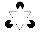
Fundamental Principles of Cognition

An alternative title for this page that I considered for a while was “Fundamental Laws of Cognition”. What you see listed below conceivably could be called “laws”, in the sense that every sufficiently complex cognitive agent necessarily follows them: it is beyond human will or consciousness to try to avoid them. But in this text I opted for the term “principles” in order to emphasize that if anyone makes a claim of having constructed (programmed) a cognitive agent, that agent should show evidence of adhering to the principles listed below. My view is that the fewer of these principles an agent employs the less cognitively interesting the agent is.

The principles listed here are not meant to be construed as exhaustive; that is, no claim is made that there exist these and no other principles in cognition. The present article should be seen as a proposal; if further principles can be proposed by others, the present list should be augmented. The present list is simply the distilled and crystallized output of the author’s research in cognitive science (see link above). Also, the given principles concern “core” (or “abstract”) cognition, not the “embodied” one; e.g., they do not cover robotics.

Contents: (alternative titles for the principles below are enclosed in parentheses)
Principle 1: Object Identification (Categorization)
Principle 2: Essence Distillation (Analogy Making)
Principle 3: Object Prediction (Pattern Completion)
Principle 4: Minimal Parsing (“Occam’s Razor”)
Principle 5: Quantity Estimation and Comparison (Numerosity Perception)
Principle 6: Association-Building by Co-occurrence (Hebbian Learning)
Principle 6½: Temporal Fading of Rarity (Learning by Forgetting)
Summary

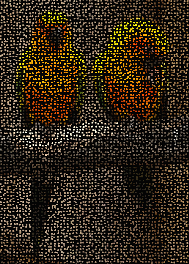
Principle 1: Object Identification (Categorization)

In his influential “Six Easy Pieces”, Richard Feynman used the description “the Mother of all physics experiments” for the famous two-slit experiment,⁽¹⁾ because the results of many other experiments in quantum physics can be traced back to the observations in the two-slit experiment. Is there any such example in cognitive science that can serve as “the Mother of all cognitive problems”? Indeed, there is. Consider Figure 1.1:

Figure 1.1. The most fundamental cognitive problem: what does this figure show?

The question in Figure 1.1 is: “What is depicted?” Most people would answer: “Two groups of dots.” ^{(2) (3)} It is possible of course to reply: “Just a bunch of dots”, but this would be an incomplete, a lazy fellow’s answer. What is it that makes people categorize the dots as belonging to two groups? It is their mutual distances, which, roughly, fall into two categories. Using a computer we can easily write a program that, after assigning x and y coordinates to each dot, will reach the same conclusion i.e., that there are two groups of dots in Figure 1.1. ⁽⁴⁾

Why is this problem fundamental? Well, let us take a look at our surroundings: if we are in a room, we might see the walls, floor, ceiling, some furniture, this document, etc. Or, consider a more natural setting, as in Figure 1.2, where two “sun conures” are shown perching on a branch. Notice, however, that the retinas of our eyes only send individual “pixels”, or dots, to the visual cortex, in the back of our brain (see a rough approximation of this in Figure 1.3). How do we manage to see objects in a scene? Why don’t we see individual dots?

Figure 1.2. Image of two sun conures (Aratinga solstitialis) perching on a branch		Figure 1.3. Conversion of previous image to “dots”, akin to retinal cells (an exaggeration; assume each dot is of one color)

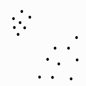
Figure 1.3 approximates the raw input we receive: each dot comes from a rod or cone (usually a cone) of the eye’s retina, and has a uniform “color” (hue, luminosity, and saturation).⁽⁵⁾ The brain then “does something” with the dots, and as a result we see objects. What the brain does (among other things) is that it groups together the dots that “belong together”. For example, most dots that come from the chest of the birds in Figure 1.3 are yellowish, so they form one group (one region); dots from the belly of the birds are more orangy, so again they “belong together”, forming another region. Both yellow and orange dots are very different from the background gray–brown dots, so the latter form another region, or regions. How many regions will be formed depends on a parameter setting that determines when dots are “close enough” (both physically and in color) so that they are lumped together in the same group. In reality, visual object recognition is much more complex: the visual cortex includes edge detectors, motion detectors, neurons that respond to slopes and lengths, and a host of other special-purpose visual machinery that has been honed by evolution (e.g., see Thompson, 1993). But a first useful step toward object identification can be performed by means of solving the problem of grouping dots together. Notice that by solving the object identification problem we don’t perceive “two birds” in Figure 1.2 (that would be object recognition), but merely “there is something here, something else there,...” and so on.

Look again at Figure 1.1: in that figure, dots belong together and form two groups simply because they are physically close; that is, their “closeness” has a single feature: physical proximity, with two dimensions, x and y. But in Figure 1.3, dots belong together not only because of physical proximity, but also because of color; thus, in Figure 1.3 the closeness of dots depends on more features (more dimensions). If color itself is analyzed in three dimensions (hue, saturation, and luminosity) then we have a total of five dimensions for the closeness of dots in that figure. A real-world visual task includes a third dimension for physical proximity (depth, arising from comparing the small disparity of dots between the two slightly different images formed by each eye), and it might include motion as an additional feature that overrules others (“dots that move together belong together”). Thus, the “closeness of dots” is a multi-dimensional concept, even for the simplest visual task of object identification.

Now let’s consider a seemingly different problem (but which will turn out to be the same in essence). In our lives we perceive faces belonging to people from different parts of the world. Some are East Asian, others are African, Northern European, and so on. We see those faces not all at once, but in the course of decades. We keep seeing them in our personal encounters, and in magazines, TV programs, movies, computer screens, etc. During all these years we might form groups of faces, and even groups within groups. For example, within the “European” face, we might learn to discern some typically German, French, Italian faces, and so on, depending on our experience. Each group has a central element, a “prototype”, the most typical face that in our view belongs to it, and we can tell how distant from the prototype a given face of the group is. (Note that the prototype does not need to correspond to an existing face, it’s just an average.) This problem is not very different from the one in Figures 1.1 and 1.3: each dot corresponds to a face, and there is a large number of dimensions, each a measurable facial feature: color of skin, distances between eyes or between the eye-line and lips, length of lips, shape of nose, and a very large number of other characteristics. Thus, the facial space has a large dimensionality. We can imagine a central dot for each of the two groups in Figure 1.1, located at the barycenter (the center of gravity, or centroid) of the group, analogous to the prototypical face of a group of people. (And, again, the dot at the barycenter is imaginary, it doesn’t correspond to a real dot.) But there are some differences: contrary to Figure 1.1, faces are probably arranged in a Gaussian distribution around the prototypical face (Figure 1.4), and we perceive them sequentially in the course of our lifetimes, not all at once. Abstractly, however, the problem is the same.

Figure 1.4. Abstract face space (pretending there are only two dimensions, x and y)

But vision is only one perceptual modality of human cognition. Just as we solve the problem of grouping faces and categorizing new ones as either belonging to known groups or becoming candidates for new groups, so we solve abstract group-formation problems such as categorizing people’s characters. We learn what a typical arrogant character is, a typical naïve one, and so on. The dimensions in this case are abstract personality features, such as greed–altruism, gullibility–skepticism, etc. Similarly, in the modality of audition we categorize musical tunes as classical, jazz, rock, country, etc.

In each of these examples (dots in Figure 1.1, pixels of objects, people’s faces, people’s characters, etc.), we are not consciously aware of the dimensions involved, but our subconscious cognitive machinery manages to perceive and process them. What kind of processing takes place with the perceptual dimensions is not precisely known yet, but the observed result of the processing has been summarized in a set of pithy formulas, known as the Generalized Context Model (GCM) (Nosofsky 1984; Kruschke, 1992; Nosofsky, 1992; Nosofsky and Palmeri, 1997). The GCM does not imply that the brain computes equations (see them in Figure 1.5) any more than Kepler’s laws imply that the planets solve differential equations while they orbit the Sun. Instead, like Kepler’s laws, the formulas of the GCM in Figure 1.5 should be regarded as an emergent property, an epiphenomenon of some deeper mechanism, the nature of which is unknown at present.

		Equation 1
		Equation 2
		Equation 3

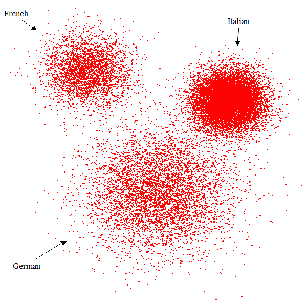
Figure 1.5. The formulas of the Generalized Context Model (GCM)

The formula in Equation 1 gives the distance d_ij between two “dots”, or “exemplars”, as they are more formally called, each of which has n dimensions, and is therefore a point in an n-dimensional space, or a so-called n-tuple (x₁,x₂,...,x_n). For example, each dot in Figure 1.1 is a point in 2-dimensional space. The w_k’s are called the weights of the dimensions, because they determine how important dimension k is in calculating the distance. For instance, if some of the dots in Figures 1.1 or 1.3 move in unison, we’d like to give a very high value to the w_k of the k-th dimension “motion with a given speed along a certain direction” (this actually would comprise not one but several dimensions); that’s because the common motion of some dots would signify that they belong to the same moving object, and all other dimensions (e.g., of physical proximity) would be much less important. Normally there is the constraint that the sum of all w_k must equal 1. Finally, the r is often taken to be equal to 2, which turns Equation 1 to a “weighted Euclidean distance”.

Equation 2 gives the similarity s_ij between two points i and j (or “dots”, or “exemplars”). If the difference d_ij is very large, then this formula makes their similarity to be nearly 0; whereas if the difference is exactly 0, then the similarity is exactly 1. The c in the formula is a constant, the effect of which is that if its value is high, then attention is paid to only very close similarity, and thus many groups (categories) are formed; whereas if its value is low, the effect is the opposite: fewer groups (categories) are formed. (How groups are formed is determined by Equation 3, see below.) Note that in some versions of the GCM, the quantity c·d_ij is raised to a power q, so that if q=1 (as in Equation 2) we have an exponential decay function, whereas if q=2 we have a Gaussian decay.

Finally, Equation 3 gives the probability P(G | i) that point i will be placed in group G. The symbol K stands for “any group”, so the first summation in the double-summation formula of the denominator says “sum for each group”. Thus, suppose that some groups have already been formed, as in Figure 1.4, and a new point (dot) arrives in the input (a new European face is observed, in the context of the example of Figure 1.4). How can we decide in which group to place it? Answer: we compute the probability P(G | i) for i = 1, 2, and 3 (because we have 3 groups) from this equation, and place it in the group with the highest probability. An allowance must be made for the case in which the highest probability turns out to be too low — lower than a given threshold. In that case we can create a new group. In practice, Equation 3 is computationally very expensive, so some other heuristic methods can be adopted when the GCM is implemented in a computer.

A question arising from Equation 3 is how we determine the very initial groupings, when there are no groups formed yet, and thus K is zero. One possible answer is that we entertain a few different grouping possibilities, allowing the reinforcement of some groups as new data arrive, and the fading of other groups in which no (or few) data points are assigned, until there is a fairly clear picture of which groups are the actual ones that emerge from the data (Foundalis and Martínez, 2007).

What’s nice about the GCM equations is that they were not imagined arbitrarily by some clever computer scientist, but were derived experimentally by psychologists who tested human subjects, and measured under controlled laboratory conditions the ways in which people form categories. Experimental observations provide strong support for the correctness of the GCM, according to Murphy (2002).

What the above formulas do not tell us is how to decide what constitutes a dimension of a “dot”. For example: you see a face; how do you know that the distance between the eyes is a dimension, whereas the distance between the tip of the nose and the tip of an eyebrow is not? Now, we people do not have to solve this problem, because our subconscious cognitive machinery solves it automatically for us, in an as yet unknown way; but when we want to solve the problem of “categorization of any arbitrary input” in a computer we are confronted with the question of what the dimensions are. There is a method, known as “multidimensional scaling”, which allows the determination of dimensions, under certain conditions.⁽⁶⁾ But more research is currently needed on this problem, and definitive answers have not arisen yet.

Opinions differ on which theory is best suited to describe the GCM. The question is: if categories are formed and look like those in Figure 1.4, then how are they represented in the human mind? This is the source of the well-known “prototype” vs. “exemplar” theory contention (see Murphy, 2002, for an introduction). The prototype theory says that categories are represented through an average value (but see Foundalis, 2006, for a more sophisticated statistical approach). The exemplar theory says that categories are represented by storing their individual examples. Many laboratory tests of the GCM with human subjects appear to support the exemplar theory, although no consensus has been reached yet. However, although the architecture of the brain seems well-suited for computing the GCM according to the exemplar theory, the architecture of present-day computers is ill-suited for this task. In Phaeaco (Foundalis, 2006), an alternative is proposed, which uses the exemplar theory as long as the category remains poor in examples (and thus the computational burden is low), and gradually shifts to the prototype theory as the category becomes more robust and its statistics more reliable. Whatever the internal representation of a category in the human mind is, the important observation is that the GCM formulas capture our experimental data of people’s behavior when they form categories.

The reader probably noticed that this section started with the question of object identification, and ended up with the problem of category formation. How was this change of subject allowed to happen? But the beauty of the First Principle is that it unifies the two notions into one: object identification and category formation are actually the same problem. It is tempting to surmise that the spectrum that starts with object identification and ends with abstract category formation has an evolutionary basis, in which cognitively simpler animals reached only the “lower” end of this spectrum (concrete object identification), whereas as they evolved to cognitively more complex creatures they were able to solve more abstract categorization problems.

The power of the First Principle is that it allows cognition to happen in a very essential way: without object identification we would be unable to perceive anything at all. Our entire cognitive edifice is based on the premise that there are objects out there (the nouns of languages), which we can count: one object, two objects... Based on the existence of objects, we note their properties (a red object, a moving object, ...), their relations (two colliding objects, one object underneath another one, ...), properties of their relations (a slowly moving object, a boringly uniform object, ...), and so on. Subtract objects from the picture, and nothing remains — cognition vanishes entirely.

A related interesting question is whether there are really no objects in the world, and our cognition simply concocts them, as some philosophers have claimed (e.g., Smith, 1996). But I think this view puts the cart in front of the horse: it is because the world is structured in some particular ways (forming conglomerations of like units) that it affords cognition, i.e., it affords the evolution of creatures that took advantage of the fact that objects exist, and used this to increase their chances of survival. Cognition mirrors the structure and properties of the world. “Strict constructivism” — the philosophical view that denies the existence of objects outside an observer’s mind — cannot explain the origin of cognition.

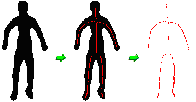
Principle 2: Essence Distillation (Analogy Making)

Simply identifying objects will not lead any cognitive agent too far. There must exist some way by which the cognitive agent does something useful with the identified objects. This cognitive ability — which is unknown whether any non-human animal possesses — is the ability to home in on the essential core of an object, event, situation, story, idea, without being distracted by superfluous details. Consider the following figure:

Figure 2.1. What’s special about the red pixels in the human figure?

Figure 2.1 shows a human figure on the left; in the middle, some pixels have been singled out in red color, shown in isolation on the right. Those pixels are not random: they have been algorithmically constructed by a program, and have the property that each one is in the “middle”, i.e., as far as possible from the “border” of this figure (the pixels that separate blackness from whiteness). The specific algorithm that identifies those pixels is not important. What’s important is that it is algorithmically possible — an easy task, in fact — both for the brain and for a computer to come up with something like the stick figure on the right. Children, early on in their development, typically use stick figures to draw people (except that they draw the most important part, the head, with an oval or circle). In music, the analogue of “drawing a stick figure” of a melody is to hum (or whistle, or play on a piano with a single finger) the most basic notes of it, in the correct pitch and duration.

When we perceive the “middle” in Figure 2.1 on the left, we disregard “uninteresting details”, such as the exact way the border pixels make up jagged lines. The human figure could include “hair” at the borders (spurious pixels), or pixels of various colors, and still we would be able to see the middle of it. But the ability to identify the “essence” of things is not confined to concrete objects; it becomes most versatile — truly astonishing — in the most abstract situations. Consider the following example:

In his book, Fluid Concepts and Creative Analogies, Douglas Hofstadter recounts an anecdotal situation, in which he was observing his just-over-one-year-old daughter, Monica, playing with a “Dustbuster” (a hand-held battery-operated toy vacuum cleaner). Monica was pushing the on–off button, having fun with the buzzing noise the toy was making. At some point, she noticed a differently shaped button on the toy, and of course tried to push that one, too. She was disappointed though, because that was the release button for the lid that held the trashbag in the toy, and after a few more failed attempts she gave up. Her father went over and showed her what the second button did, but little Monica wasn’t impressed much.

Suddenly, her father had a flash in his memory of something that happened in his childhood. He had learned, as an eight-year-old, to apply various arithmetic operations on numbers, and one of the operations he was enjoying very much was the exponentiation. (I suspect that his own father, Robert Hofstadter — the 1961 Nobel laureate in physics — must have had played no small part in that.) One day, young Doug noticed the math notation on one of his father’s physics papers, and was attracted by the ubiquitous use of subscripts. Being familiar with the wonders of superscripts, he jumped to the conclusion that subscripts must be hiding a similarly wonderful world in arithmetic. He was disappointed, however, when he asked his father and was told that subscripts are simply used to distinguish one variable from another (Hofstadter, 1995a).

Hofstadter’s is a quintessential (yet astonishing) example of an analogy. There are two analogous situations that are mapped, and there is a common core, an essence that remains invariant between the two situations. In this example, the essence comprises a father–child relation, a “toy” with a single feature with which the child has had fun playing, a second similar feature on the toy that’s suddenly discovered by the child, and a disappointment after the child is informed by the father that this second feature does nothing very interesting.

However, when an analogous situation comes to one’s mind, one does not usually think consciously of the essence of both situations. It’s possible to do it after careful examination, as I did in the previous paragraph, but, unless we search for it explicitly, the common core eludes us almost always. This core, the essence, is as subconscious as the middle pixels in Figure 2.1, which we do not imagine consciously unless we are asked explicitly to do so. Yet the core must exist, otherwise we would be unable to draw stick figures, or to make analogies like the above.

And it’s not just a seemingly exotic ability (“analogy making”) which is involved. The ability to perceive the essence and disregard the inessential details allows us to think of concepts such as “triangle” and “circle”, without caring about the thickness of the lines that make up such geometric objects, or even about the lines themselves. Thus, we can abstract those concepts fully, and talk of a “triangle-like relation of people”, or “my circle of friends”. The ability to perceive the core of things led the ancient philosopher Plato to claim that there is a deeper, immaterial world of essences, and that when we talk about a circle (or a table, or anything at all) we have access to that ideal object, whereas our material world supplies us with a lot of extra, inessential details. This was Plato’s famous Theory of Forms, which influenced Western thought for two and a half millennia. Although today Plato’s theory does not have the influence it once had, it shows that when the ancient thinker tried to find what’s fundamental in a mind, he hit the nail on the head. Other, present-day thinkers, such as Douglas Hofstadter, claim that analogy-making is at the core of cognition (Hofstadter, 2001). This claim is difficult to understand, because the term “analogy making” typically invokes to the uninitiated boring logical puzzles of the form “A is to B as C is to what?” But, beyond logical puzzles, we use and create new analogies (or metaphors, in Lakoff’s terms — see also the fourth principle) all the time, even as we are talking. If our thoughts remained constrained in what can only be immediately seen, if we were unable to abstract by extracting the core of concepts, we would still be living in a very primitive world.

Earlier, I suggested that only humans have this ability. However, it can be surmised that when chimpanzees use a stick to “fish” termites out of a hole they do not perceive the stick as what it is (a broken piece of a tree or bush), but as an elongated solid object, which is the essence of a branch that’s important for the task they want it for. Every use of something as a tool — be it a crude stone or a sophisticated Swiss knife — makes use of the object not as what it is (a chunk of rock, a piece of metal and plastic), but as what its deeper essence can help the tool-handler achieve. Even the use of toys can be said to have the same cognitive function as that of tools, and cognitively complex mammals and birds are known to use a wide array of toys.⁽⁸⁾

Figure 2.2. A cute young chimp girl (Pan troglodytes) using a stick and a feather as toys

Some researchers in cognitive science and artificial intelligence have announced the construction of software that, supposedly, can “discover analogies”. For example, they say that, given the ideas of a solar system and an atom with its nucleus and orbiting electrons, their programs can discover the analogy between the two structures. Such claims are largely vacuous. (I prefer to avoid making explicit references here, but see Hofstadter, 1995b, for another critical view of such approaches.) What they mean is that after someone (a person) has codified explicitly the structure of a solar system, plus that of an atom, there comes their program to “discover” that there is an analogy there. But the whole problem rests on our ability to discover spontaneously the two similar structures, as in Hofstadter’s example, above! Hofstadter didn’t think “Let’s make an analogy now! — uh, what is the core of the situation we have over here?” Neither did he think of finding the core, nor did he search consciously for a match between the core and something in his memory. It all happened automatically. If someone tells me, “Here are two structures, find if there is an analogy between them and explain why”, the problem is nearly solved — thank you very much. How do we zero in on the essential and match it with something that shares the same essence spontaneously? That is the crucial question in research in analogy-making.

My answer is that analogy making happens spontaneously and subconsciously as follows: (1) when input is perceived, it is stored in long-term memory through a representation that already includes its extracted core, because core extraction happens automatically; (2) the core of that representation can be seen as a “dot” (in the sense of the First Principle) that’s located in an abstract multi-dimensional conceptual space; (3) when a new input is perceived, it of course goes through the same process of core extraction; (4) the new core (the newly perceived one) is another “dot” that’s located in the same abstract multi-dimensional conceptual space as the old “dot” (old core); (5) if the new core is “close” (as per the First Principle) to the old core, then the old core is activated, and through its activation we remember the entire old concept. Thus, the new concept invokes the old concept. Why does this process have to be done by using cores and not the entire representations? Because it is computationally much simpler to find that the two cores match well enough (since the cores contain only the essential features, and here “essential” means “those that matter”), rather than to compare and match entire representations, which contain perhaps dozens of irrelevant features. If the reader is further interested in this issue, I discuss it more thoroughly in this paper (2013).

The Second Principle is implemented in Phaeaco by extracting the core of the visual input, as shown in Figure 2.1, and using that core to represent the structure of the input internally, as well as to store it in long-term memory. If visual input with a similar core structure appears later, Phaeaco will match the two structures and mark them as highly similar, even if they differ in their details (and will do this automatically, without anyone asking it explicitly to do so at any time). Whether this ability can be augmented in the future so that Phaeaco becomes capable of extracting the core of more abstract entities — such as thoughts and ideas — remains to be examined.

Principle 3: Object Prediction (Pattern Completion)

Consider the following figure:

Figure 3.1. What do you see here?

Many readers are undoubtedly in a position to tell not only that Figure 3.1 shows “a face”, but also which particular individual is depicted. Yet the figure doesn’t even show a face, but only various features of one: an eye, a nose, part of the forehead, some hair. These are more than enough, however, for everyone to recall the concept “face”, and for some (many, perhaps) to recall the more specific concept “Albert Einstein”. What happens is that we recall the whole on the basis of some parts of it. Now consider the following:

2, 4, 6, 8, 10, 12, 14, ...

Figure 3.2. What is the next number in sequence?

It doesn’t take more than a few seconds to realize that the sequence in Figure 3.2 is the beginning of the positive even numbers, and thus to predict that the next number in this sequence should be 16. The appropriate term in this context is “inductive reasoning”, i.e., given some examples, we use them to figure out inductively the underlying rule (“even numbers”, in Figure 3.2), and by extrapolation we predict the future instances.

Figures 3.1 and 3.2 show examples of “pattern completion”, a very important cognitive ability. The difference between the two examples is that the information in Figure 3.2 is sequential, whereas that of Figure 3.1 is not: we could be given any part, or parts, of Einstein’s face and still predict the rest (or simply reach the concept “face”, if the information is not enough to reach “Einstein”). In contrast, the order matters in the case of the input in Figure 3.2. Whether the object prediction (or pattern completion) task is sequential or not depends on the input modality. Visual and haptic (tactile, of touch) information is largely non-sequential (e.g., if an object fits in our palms we can usually tell what it is with closed eyes without scanning it sequentially); whereas auditory information is necessarily sequential, which makes the perception of language and music a sequential task; e.g., having heard part of a sentence, we can often predict approximately what the next few words will be (which causes people sometimes to adopt the annoying habit of interrupting others, feeling they don’t need to wait for the idea to be fully spelled out); also, having heard part of a familiar piece of music, we can predict usually exactly what the continuation will be, because there is hardly any variation in the way a familiar piece is played. (If there is, then we perceive it as an out-of-tune case.)

Just as in the cases of the previous principles, the ability to predict and complete patterns is not uniquely human, but originated in animal cognition. Indeed, it is vitally important for survival. Consider that an animal can be confronted with the sight in Figure 3.3:

Figure 3.3. Pair of jaws floating on the river?

The animal would perhaps live a little longer if it could “predict” that it’s not just a pair of jaws floating on the river that are involved, but that there is an entire hippo underneath. Sequential prediction is also within the reach of animals, as experiments in animal psychology have shown.

The principle of pattern completion is directly at work in cases where the context suggests us to complete or interpret missing or ambiguous information one way or another. Consider the following well-known ambiguous drawing:

Figure 3.4. The ambiguous letter in the middle can be seen as either an “A” or an “H”

If we read horizontally in Figure 3.4, we see the word “THE”, thus interpreting the middle letter as “H”; but if we read vertically, we see the word “CAT”, interpreting the middle letter as “A”. In this case, the context helps us interpret the ambiguous figure in one way or another, so we supply the missing information in different ways. In other cases, the context becomes an essential aid to complete the missing information, such as when you read any text consisting of long sentences: you don’t see each individual letter as you read, as evidenced by experiments that track the saccades of the eyes (rapid eye-movements); instead, you jump from word to word, often skipping over entire small words, and fill out the missing information by means of what you expect to see, i.e., by means of the contcxt. (If you spotted the typo in the last word of the previous sentence, congratulations; if you missed it, you interpreted the c as an e, aided by the context.)

Again, there is the question of the implementation of pattern completion. How does the brain achieve it, and how can we implement it in a computer? Work in neural networks has shown that it is relatively easy to implement a rudimentary form of pattern completion in computers, assuming the invariance of the input; i.e., the network should not fail entirely if the input is shifted, rotated, or zoomed to some extent. The brain, however, does not assume the invariance of the input, but achieves it. The exact way is not precisely known yet, but this neurobiological question does not concern us here. Since it is not yet known how to achieve input invariance in neural networks, and because computer hardware is based on an entirely different architecture compared to the neuronal one, other computational approaches can also be of value. In Phaeaco there is a front-end and a back-end visual processing system. The back-end (which is not sharply separated from the front-end) is responsible for building internal representations of whatever is seen. Now if, while the representation is being built (but while it is not complete yet), a concept is reached and activated sufficiently in long-term memory, then the back-end has the ability to conclude the equivalent of: “Fine, I know what I’m seeing, I don’t need further confirmation”, and it effectively stops the front-end procedures from further examination of the actual input (in order to save computer cycles; a biological organism wouldn’t need to do that). This is the way Phaeaco “sees without seeing” everything that’s visible — a very important ability for pattern-completion.

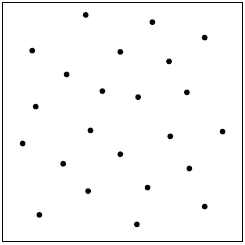
Principle 5: Quantity Estimation and Comparison (Numerosity Perception)

Consider the following figure:

Figure 5.1. How many dots do you see, roughly, without counting them?

Everybody can come up with a rough estimate of the number of dots in Figure 5.1, without resorting to counting. Although estimates might vary, few people — if any — would claim they see fewer than 10 dots, or more than 50.

The ability that allows us to come up with an estimate of the quantity of discrete (countable) objects is the perception of numerosity (i.e., of the number of things), and this ability obeys certain regularities, which are discussed below.

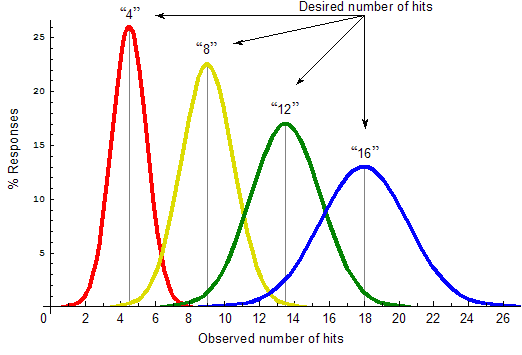
If, for example, only three dots are flashed in front of our eyes, even for a split-second, our estimate will be nearly always accurate: three dots. If, however, 23 dots are shown (as in Figure 5.1), then it is quite unlikely that we’ll come up with “23” as an answer, no matter for how long we see them (provided we don’t resort to counting); more likely, our estimate will be somewhere between 15 and 30. But if we repeat the experiment many times, then the average estimate will approach the number 23 (provided we receive some prior training in dot-number estimation; otherwise — without training — our average estimate might converge to a somewhat different number). Last, but not least, if 100 dots are shown, our estimate will vary in a larger interval: we might report numbers anywhere between 50 and 150 (for instance — I’m only guesstimating the interval).

How do we know the above idea is true? Experiments that verify this idea were not done on people, but on rats! Yes, animals as cognitively simple as rats are in a position to estimate the number of things. In an experiment done by Mechner in 1958, and repeated by Platt and Johnson in 1971, hungry rats were required to press on a lever a number of times before pressing once on a second lever, which would open a door to a compartment with food (Mechner, 1958; Platt and Johnson, 1971). The rats learned by trial and error that they had to press, for instance, eight times on lever A, before pressing once on lever B to open the door that gave them access to food. Each rat was trained with a different number of required presses on lever A. To avoid having rats press on the desired lever B prematurely, the experimenters had the apparatus deliver a mild electrical shock to the poor rat, if the animal hurried too much. (Without this setup the rats tended to press on B immediately, failing to deliver the required number of hits on A.) Anyway, the rats never learned to be accurate, because, unlike us, they cannot count; they only estimated the number of required hits on lever A, and their estimates, summarized in Figure 5.2, were very telling of what was going on in their little brains.

Figure 5.2. Rat numerosity performance (adapted from Dehaene, 1997)

To understand the graph in Figure 5.2 concentrate first on the red curve. This curve describes the summarized (statistical) achievements of those rats that learned the number “4” (you see it marked on the top of the red curve). The average value of this curve (its middle, that is) is not exactly at 4 on the x-axis, but somewhere near 4.5. This is because the rats overestimated slightly the number 4 that they were learning: besides 4 hits on lever A, they gave some times 5 hits, other (fewer) times 3 hits, some times 6 hits, and so on. Each point of the red curve gives the probability that a rat would deliver 2 hits, or 3, 4, 5, etc. The same pattern is observed with the other curves (yellow, green, and blue), which summarize the estimates of other rats, learning different numbers (8, 12, and 16, respectively). We see that in all cases the rats overestimated the number of hits: for example, those who were learning “16” hit lever A an average of 18 times. They probably did this because they were “playing it safe”: due to the mild electrical shock, they avoided hitting on B prematurely; on the other hand they were hungry, so they didn’t want to continue pressing on A for too long.

Why should we be concerned with rats? Because it’s easier to perform such experiments on them: first, it is inadmissible to deliver electrical shocks to humans, and second, humans can cheat, e.g., by counting.⁽⁹⁾ The observations regarding the perception of numerosity, however, should apply equally to rats and humans. See, numerosity perception is not mathematics; it has nothing to do with our human-only ability to manipulate numbers in ways that we learn at school. We share the mechanism by which we perceive numerosity with many other, cognitively capable animals, including rats, some birds, dolphins, monkeys, apes, and many others.

One observation in Figure 5.2 is that the larger the number that must be estimated, the less accurate its estimate is, and the distribution of estimates is given by those Gaussian-like curves. Note that the curves are not exactly Gaussian: they should be skewed slightly towards the left (though this is not shown in Figure 5.2), especially those that correspond to smaller numbers.

Second, there are regularities when we compare quantities; that is, when we are presented simultaneously with two boxes, each with a different number of dots:

In other words, it is easier to discriminate between 5 and 10 dots than between 5 and 6 dots. Okay, this is obvious. But there is also this result:

This means that it is easier to discriminate between 5 and 6 dots than between 25 and 26. Obvious, too, but only when you think a bit about it.

Both of the above observations can be easily verified on human subjects, who answer faster that there is a difference when it is easier to discriminate the numbers.

It is possible that we use the same ability to perceive the difference in size of arbitrary shapes. Consider Figure 5.3:

Figure 5.3. Which of the two islands is larger?

In Figure 5.3, two islands of the Aegean Sea are depicted: Andros on the left, and Naxos on the right. Which one appears larger? Although a search in the Internet will reveal that Andros (374 km²) is smaller than Naxos (428 km²), the same can be concluded by merely looking at them carefully, for some time. Perhaps we achieve this by having a sense of the number of “pixels” that belong to each island (e.g., a first discretization of them in “pixels” is provided by the cones of our retinas), an idea schematically depicted in Figure 5.4.

Figure 5.4. Discretization of the area of the islands (exaggerated, low resolution)

But what kind of mechanism can account for the above observations?

Stanislas Dehaene supported the accumulator metaphor to model these observations (Dehaene, 1997). The accumulator metaphor says that when you are presented with a display that has, say, dots, each dot does not add exactly 1 to some accumulator in your brain, but approximately 1. Specifically, a quantity that has a Gaussian distribution around 1 is added. That is, instead of 1, a random number from a Gaussian (“normal”) probability distribution N (1, σ₀) is generated, and is added to the accumulator. Obviously, the smaller σ₀ is, the more accurate the estimation will turn out to be. If a person can make better estimates than another one, this is probably because the σ₀ that the first person’s cognitive apparatus uses is somewhat smaller than the second person’s. But, in the end, it’s all probabilities, so no one is guaranteed to always estimate better than someone else. Dehaene says that a quantity of “approximately 1” could be achieved in the brain with the spurt of a chemical, the exact quantity of which cannot be precisely regulated.

Does the accumulator metaphor explain the experimental observations? It does, and neatly so. If you add n Gaussian random numbers from N (1, σ₀), what you get is again a Gaussian random number, with mean μ_Σ = n and standard deviation σ_Σ = σ₀. These two numbers, μ_Σ and σ_Σ, determine the location and shape of the colored curves of Figure 5.2, the formulas of which are given below (depending on n):

Equation 5.1. Formula for numerosity perception of n entities

Thus we have a mathematical description of the curves that the rats (and other animals, such as humans) produce. (This is of course an approximation: recall that for small numbers the curve is actually skewed to the left; also, Equation 5.1 allows negative numbers, which are of course impossible; but, generally, the approximation is very good.) The shape of these curves (see again Figure 5.2) explains why the fewer the entities, the more accurate our estimate of their number is: it’s because with fewer entities (small n) the Gaussian bell-like curve is narrower, and so there is a high probability that the random number produced will be close to the mean n.

What about the comparison of numerosities? How can we model mathematically observations concerning how fast people discriminate among different numerosities?

Those observations, too, can be understood by the accumulator metaphor. You see, if you have to distinguish between 5 and 6, you deal with two quite narrow Gaussian curves, with small overlap. When the overlap is small, your confusion is low. But if you must distinguish between 25 and 26, the Gaussians for those two numbers will overlap nearly everywhere. Large overlap means high confusion. Okay, so the confusion is explained qualitatively by the curves. But what about the reaction times to discriminate among different numerosities? Those can be modeled mathematically by something known as “Welford’s formula” (Welford, 1960):

Equation 5.2. Welford’s formula for reaction time RT to discriminate among a large (L) and a small (S) numerosity

The reaction time RT in Welford’s formula depends on L, the larger of the two numerosities, on S, the smaller of the two, and on some constants, such as a, which is a small initial overhead before a person “warms up” enough to respond to any stimulus. Equation 5.2 should not be construed too literally, however. For instance, if L = S, RT is not defined, or we may say the formula suggests that the person will wait to infinity (because dividing by zero might be thought of as producing infinity); obviously, no person will be stuck forever, like a robot. In general, for large L and S Welford’s formula is not very accurate. But, approximately, it’s good enough.

Welford’s formula, proposed in 1960, is an elaboration of an even older formula, known as the Weber – Fechner law. That’s a law stated in the 19th century, and says that if the stimulus has magnitude m, what we sense is not m itself, but a quantity s which is proportional to the logarithm of m, like this: s = k·log(m) (k is again a constant). The logarithm explains how, for example, we can see very well both under the light of a bulb, and under bright sunlight, which is thousands of times brighter than the bulb light in absolute terms.

All these formulas are fine, but they don’t tell us what’s special in human perception of numerosity, which doesn’t occur in other animals.

Well, as usual, human cognition went one step further. Instead of perceiving the magnitude of only explicit discrete quantities (such as dots), we can perceive the magnitude of symbolic quantities as well. For example, human subjects can be asked to discriminate quantities by looking at numerals such as 5 and 6, in their common (Arabic) notation; or, to discriminate among letters, such as e and f, assuming that each letter stands for its ordinal location in the alphabet. In all such cases, the accumulator metaphor and Welford’s formula are still valid. This suggests that every comparison of quantities or sizes, however abstract, is governed by the principles for numerosity perception discussed in this section.

The phrase “however abstract”, above, is crucial. By means of our numerosity perception we can have a sense of the magnitude of such quantities as:

• How many times we ate Chinese food within the past year (assuming we don’t consume Chinese food on a daily basis, nor that we have some aversion to it).

• How many times our arms move back-and-forth while brushing our teeth.

• How many times the word “cognition” appears in this document, and that this number must be larger than the number of occurrences of “fundamental”.

For none of the above examples do we have an exact number to report (under normal circumstances), nor have we thought of counting while the events were taking place. Instead, we have a “sense of magnitude”, and that’s what this principle is about.

Principle 6: Association-Building by Co-occurrence (Hebbian Learning)

That animals can form associations is well known. In fact, this used to be considered the most solid finding in animal psychology in the beginning of the 20th century (cf. Pavlov’s experiments with dogs salivating after hearing a bell ringing), and formed the basis of the stimulus–response behaviorist view of cognition. Since then, the behaviorist view has fallen into disrepute in cognitive science (though it still has some avid fans in the domain of biology), because it failed to explain observations in human cognition. Its core idea, however, still appears in cognition, in what is known as “Hebbian learning”, according to which, when two neurons are physically close and are activated together, some chemical changes must occur in their structures that signify the fact that the two neurons fired together (Hebb, 1949). Psychologists and cognitive scientists generalized this idea, taking it to mean that whenever two percepts are repeatedly perceived together, the mind forms an association between them, so that one can invoke the other. If they are perceived sequentially, the first will invoke the second, but not vice versa; but if their perception is simultaneous, e.g., as when we repeatedly see two friends appearing together, then the presentation of either one will invoke the concept of the other. (If only one of the friends greets us one day, we are tempted to ask how’s the other one doing.) See Figure 6.1 for a well-known example.

Figure 6.1. Which “friend” does Mr. Hardy bring to your mind?

But the example that follows is a “live demonstration” of the fact that animals build associations by co-occurrence. The other day I happened to be in the zoo of Athens, Greece (the Attica Zoological Park), next to the cage of a cockatoo. Cockatoos are parrot-like birds, and, like many parrots, they can learn to “talk”. This one, besides being good at talking, was also very fond of being petted. No, not just fond of it, it demanded to be petted by the visitors. I inserted one finger through the metallic grid of its cage, and the bird, delighted, lowered its head, allowing me to caress its neck and body under the wing (which it lifted, so that I could caress it there!). Then when I withdrew my finger and was about to leave, I heard it saying: “Ti kánis?” which in Greek means, “How are you doing?” Wow! — I thought — this bird can talk, too! So I went back and petted it some more. This scenario was repeated twice, and each time the bird said “Ti KAnis?” while I was distancing myself from its cage. The third time, I thought, I should record this. I asked a friend who was with me to pet the bird while I was using my camera to take a movie of it, and when we distanced ourselves, sure enough, the bird blurted out another “Ti kánis?” You can see the movie below:

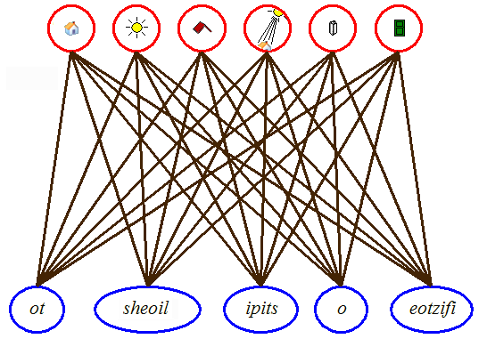
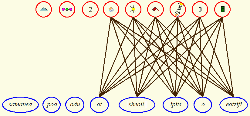
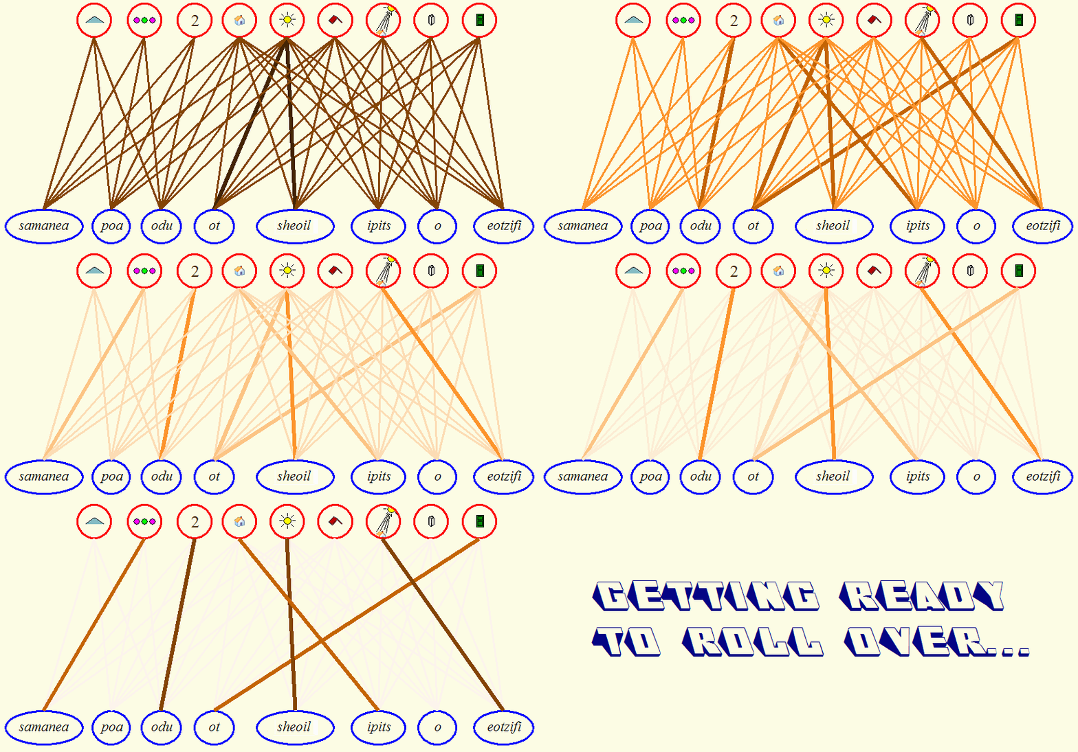
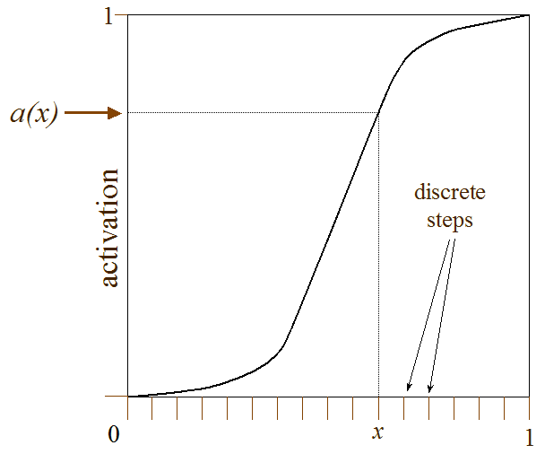
Why did the bird do that? Well, the “Ti kánis?” effectively meant for the cockatoo: “Come back here! (I want more petting!)” The bird had noted, by trial and chance alone, that whenever it uttered something the visitors who were just leaving would come back with a “Wow!”, and pet it some more. The bird probably used this phrase, “Ti kánis?”, from the very beginning, and formed an association between its utterance and the coming back of people, which is what it wanted.

In this example we see an amazing ability for an animal, which we usually ascribe to people only. Out of all the events that were taking place while people were distancing themselves from its cage, the bird singled out the one and only event, its uttering of “Ti kánis?”, which would effectively bring the people back to it. The first time that this happened, it ought to have happened by chance, for the cockatoo has no way of knowing that something it said would have a felicitous outcome. It simply noticed the co-occurrence, perhaps from the first time; then it repeated it, and got convinced that doing this, results in that. The last repetition which is always a failure (because people do have to leave its cage at some point) did not make it “forget” the association. Our cockatoo reminded me of scientists of older times who tried various medicines to cure a disease, and when they observed that the disease was indeed cured they tried to figure out which chemical it was that did the trick, until they came to an “Aha!”-moment, “It’s this substance!” Except that, what we people can sometimes do with the help of consciousness, and sometimes unconsciously, birds and other animals can do unconsciously only.

Note that, so far, Hebbian learning can be seen as merely another application of the pattern-completion principle. However, the sixth principle is about a generalization of Hebbian learning, in which a percept from an entire set can be associated simultaneously with one or more percepts from another set, without anyone telling us explicitly which percept must go with which one. Here is an example:

Suppose you are an infant; you’ve just started learning your native language, in the automatic and unconscious way all infants do. You are presented with images of the world — things that you see — and words of your language, which, more often than not, are about the things you see, especially when adults speak directly to you. The problem that you have to solve — always automatically and subconsciously — is to figure out which word roughly corresponds to which percept in your visual input. (Let’s assume you’ve reached a stage at which you can identify some individual words.) The difficulty of this problem lies in the fact that there is a multitude of visual percepts every time, and a multitude of linguistic tokens (words, or other morphological pieces, such as plural markers, possessives, person markers, and so on). How do you make a one-percept-to-one-token correspondence when what you’re given to begin with is a many-to-many relation?

The following solution makes several assumptions that are idealizations; i.e., the real world is more complex. But, as usual, we arrive nowhere if we confront the real world in its full generality immediately. Some simplifications must be made, some corners must be cut, to be able to see first the basic idea; afterwards, more complications can be added with an eye toward testing whether the basic idea still works. So: suppose that the input — both visual and linguistic — is given to you in pairs of one image, and one phrase that’s about that image, as in Figure 6.2.

o sheoil eotzifi ot ipits

Figure 6.2. An image (red, visual input) paired with a phrase in an unknown language (blue, linguistic input)

Looking at the image, you can identify some visual percepts; whereas listening to the phrase, you can identify some linguistic tokens. But you have no clue which visual percept to associate with which linguistic token. So, being clueless as you are, why not making an initial association of everything with everything? The following figure depicts just this sort of idea.

Figure 6.3. Forming associations between every visual percept and every linguistic token

The visual percepts are lined up on the top row in Figure 6.3, and the linguistic tokens on the bottom row, in no particular order (to emphasize that there need be no order for this algorithm to work). The percepts of the visual set (top row) are assumed to be: “house”, “sun”, “roof”, “shines”, “chimney”, and “door”. Note that these are supposed to be the percepts you happened to perceive at this particular presentation of the input; a presentation of the same input at a different time might result in your perception of somewhat different percepts; however, the algorithm described here is not sensitive to (is independent of) such variations in the input.

So every percept has been associated with every token in Figure 6.3; not a very useful construction so far, but the world continues supplying you with pairs of images and phrases. The next example is shown in Figure 6.4.

o sheoil ot eotzifi samanea poa odu onbau

Figure 6.4. Another pair of visual and linguistic input

Now you have different visual percepts from this image, and different tokens from the phrase. But, generally (from time to time), there will be some overlap — you can’t continue receiving different input elements all the time because your infant’s world is finite and restricted. So, the rows (sets) in the next figure (6.5) are supposed to contain the union of your visual percepts, and the union of your linguistic tokens — except that because the horizontal space on the computer screen is limited, only a sample of the new percepts and tokens of the two sets (rows) are shown.

Figure 6.5. Some new visual percepts and linguistic tokens are added to each set (row)

The percepts “mountain”, “between”, and “two” have been added on the visual set (top row), and the tokens “samanea”, “poa”, and “odu” on the linguistic set (bottom row), in Figure 6.5. (Everything else that you perceived, both visually and linguistically, is assumed to be there, just not shown for lack of horizontal space.)

Now we can do exactly the same thing as we did before: associate every percept from the visual input in Figure 6.4 with every linguistic input token in the same figure. The result is shown in Figure 6.6

Figure 6.6. The new visual percepts are associated with the new linguistic tokens

What happened in Figure 6.6 is that some of the original associations did not appear again (the majority of them, actually); so the strength of those associations faded somewhat, automatically (shown in lighter color). Why? Well, assume that this is a feature of associations: if they are not reinforced, and time goes by, their strength decreases. (How fast? This is an important parameter of the system, discussed later.) But some associations (a few) were repeated in the second input, and those associations increased their strength somewhat (shown thicker and in darker color).

This situation continues as described: more pairs of images and phrases arrive, and associations that are not reinforced fade, but those that are repeated in the input receive reinforcements and become stronger. The following figure is designed to show the process of this simultaneous fading and reinforcement over a number of presentations of pairs of input (image + phrase).

Figure 6.7. An animated sequence showing the building of associations between some percepts and some tokens

Figure 6.7, above, retains the same set of percepts and tokens as shown earlier in Figure 6.6. The reader must assume that these sets keep growing, because it is always the unions of percepts and tokens that the algorithm works with. But for visualization purposes the sets in Figure 6.7 have been truncated to a fixed size.

The bottom line is that in the final of the frames shown in Figure 6.7 the “correct” associations have been found. I put “correct” in quotes because whether they are truly correct or not depends on how consistent the correspondence was between images and phrases. But even if they are wrong — and some of them are bound to be — time will fix them: the wrong associations are not expected to be repeated often (unless a malevolent teacher is involved, but here we assume a normal situation, in which there are neither malevolent nor very efficient and capable teachers, just the normal input that babies are usually confronted with). So, those associations that are not repeated often, even if they somehow manage to become strong, will eventually fade. Given enough time, only the right ones will survive from this weeding process.

For the above algorithm to really work some extra parameters and safety switches must be set. Specifically, once an association exceeds a sufficient threshold of strength, it must become harder for it to fade, otherwise everything (all associations) will drop back to zero if input does not keep coming, and the mind will become amnesic, forgetting everything it learned. Also, the way strengths increase and fade must be tuned carefully, following a sigmoid function, shown in Figure 6.8.

Figure 6.8. The sigmoid function according to which associations are reinforced and fade

Function a(x), shown in Figure 6.8, must have the shape of a sigmoid for the following reasons:

• a must be increasing strictly monotonically, otherwise the motion of x along the x-axis would not move a(x) in the proper direction.

• The curve must be initially increasing slowly, so that an initial number of reinforcements starting from x = 0 does not result in an abrupt increase in a(x). This is necessary because if a wrong association is made, we do not want a small number of initial reinforcements to result in a significant a(x) — we do not wish “noise” to be taken seriously.

• Conversely, if x has approached 1, and thus a(x) is also close to 1, we do not want a(x) to suddenly drop to lower values; a must be conservative, meaning that once a significant a(x) has been established it should not be too easy to “forget” it.

• Having established that the initial and final parts must be increasing slowly, there are only few possibilities for the middle part of a monotonic curve, hence the sigmoid shape of function a.

All these are explained in further detail in Foundalis and Martínez (2007), to which the reader is referred if interested in the details. The same publication discusses a generalization between this sixth principle (the building of Hebbian-like associations) and the first principle (categorization): it is suggested that the same mechanism that is responsible for Hebbian-like association building might also be responsible for categorization. Here, however, we don’t need to delve into that generalization, which, after all, is only a possibility — no experimental evidence so far suggests that the human brain really uses a single general procedure. The generalization is more interesting for computational purposes, when implementing cognitive agents: although nature has been free — by means of natural selection — to use any mechanism that works, engineers who attempt to build cognitive systems in computers are not bound to replicate nature’s solutions.

Principle 6½: Temporal Fading of Rarity (Learning by Forgetting)

This principle is numbered 6½ to emphasize that it is not really new, but a deeper mechanism that already appeared in the discussion of the sixth principle. This mechanism, however, can also operate independently of the 6th principle, and is responsible for some of the additional learning that our cognitive systems can afford.

Once again, suppose you are an infant. Linguistic input comes to you mainly from the speech of adults. However, what you receive as input is only a tiny fraction of what your native language is in a position to generate, in principle. Therefore, you must possess some generalization mechanism that is capable of generating more sentences and word-forms than you have ever heard. For example, you hear that the past tense of “jump” is “jumped”, the past of “tickle” is “tickled”, the past of “laugh” is “laughed”, and so on. From such examples, you must be capable of inferring that the past tense of “cackle” must be “cackled”, even if perhaps you never heard the form “cackled” before. Similarly, you must be capable of putting words in ways that make sentences that you never heard before. (This observation, often called the argument from the “poverty of the input”, is used as an argument to show that human cognition must include some innate linguistic mechanism capable of coming up with such generalizations, and not simply reproducing what has already been heard.)

Fine. But every language is tricky. In English, for example, you might naturally conclude that the past tense of “go” is “goed”, and children have been observed to actually make such mistakes. The question is, how do children learn the correct form, “went”, if nobody corrects them explicitly? You might think that if an adult hears the child saying “goed”, the adult would respond, “No! You shouldn’t say ‘goed’; you should say ‘went’!” But there are two problems with this idea: first, it has been observed that many children (perhaps the majority) do not learn by being corrected — they simply ignore corrections. And second, to correct the speech of little children is primarily a Western habit. There are cultures in which adults never direct their speech to children, reasoning that the child will not understand the adult language anyway. In such cultures, the child has to learn the language — and does succeed in learning it — from whatever adult speech reaches the child’s ears. In other cultures, correcting children is simply not a common practice. So, how do children manage to un-learn the wrong generalizations that the input occasionally leads them to make?

Simple: by means of principle 6½. This principle, which already appeared as part of principle 6, says that it is not disastrous if wrong concepts are formed, or wrong connections between concepts are established, because the wrong concept or connection is bound not to be repeated too often in the input (otherwise it would be right, not wrong). Thus, the wrong connection will fade in time (automatically as time goes by, as explained in the sixth principle), and, given enough time, the wrong concept will become inaccessible; and an inaccessible concept is as if it does not exist. For example, the form “goed” is not one that will appear often in the child’s linguistic input — except rarely from other children who made the same wrong generalization. Thus, assuming there is a connection that reaches the form “goed” when the past tense of “go” is required, the strength of this connection is bound to fade in time because there will not be enough reinforcement from the input. Instead, the correct form “went” will be repeated many times, and the child will form the correct connection at some point, eventually losing the ability to reach the wrong form “goed”, because the strength of the connection to it will be too weak for any significant amount of activation to reach it and select it as the past tense of “go”.

What was just described regarding linguistic input generalizes to any situation in which we learn information by being presented with various examples, which we are expected to generalize in order to use effectively. The following figure shows the general idea:

(a)	(b)

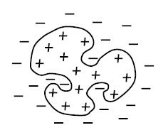
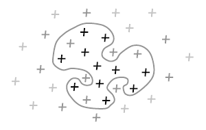
Figure 6.9. (a) Both positive and negative examples are available; (b) Only positive examples are available

Figure 6.9 (a) shows an unrealistic situation in which both positive and negative examples are available. This is called “supervised learning” in the relevant literature, because there is assumed to exist a “tutor” who tells the learning agent: “Look: this is a good example of what I expect you to learn”, and then “But now look: this is a counter-example of what you should learn”. What’s unrealistic is the existence of the tutor who chooses counter-examples (minuses (–) in Fig. 6.9.a) in addition to the positive ones (+). If such a tutor were available, the extent of the concept that must be learned (curved border) could be easily determined. But what usually happens in reality is “unsupervised learning”, in which there is no tutor, and no confirmation of whether what was learned was right or wrong. Figure 6.9 (b) shows positive examples only (+), but which, according to principle 6½, do not have a permanent life. Those that are not repeated often are — quite likely — the wrong ones, and as such, after fading sufficiently, are excluded from the extension of the learned concept. (The border of the concept is shown in gray color to reflect the fact that it changes dynamically while the concept is being learned.)

Note that what appear as grayed plus-signs in Fig. 6.9 (b) don’t have to be wrong information, but simply information that happened not to be reinforced by repetition. In this way the human mind stays always with current knowledge. Assuming that the capacity of the human brain is finite, if all information were retained indefinitely, the brain’s capacity would be exceeded at some point (probably early on in life), and we would never learn anything new. Thus, forgetting is a natural component of learning, rather than a malfunction of the human memory system.

For further information on learning by forgetting, and about the way this principle has been implemented in Phaeaco, the reader is referred to Foundalis, 2006 (§9.4.2, pp. 264–269).

Summary

A number of principles (or “laws”) of cognition were presented, seven in total (I prefer to count them as 6½), which suggest that, although cognition emerged as an evolutionary property of biological organisms, it stands alone as a discipline, independent of its biological underpinnings. To corroborate this idea, in each principle I made references to the way the principle has been implemented in Phaeaco, a programmed cognitive system, thus suggesting that cognition can be simulated computationally in a manner independent of biology. I firmly believe that, one day, it will become possible to build computing systems that think like (or perhaps even better than) human minds, just as it became possible to build machines that fly like (actually better than) birds. But before we were able to build internal combustion engines, install turbines in jets, and make them take off the ground, crossing over oceans and accommodating thousands of passengers every day, we had developed a solid theory of classical mechanics, fluids, and aerodynamics. It is in the spirit of building just such a theoretical foundation of cognition that the above principles are discussed, making the claim that they must be necessary, but avoiding the claim that they must be sufficient.

Acknowledgments

I would like to thank my friend, Prof. Alexandre Linhares, for bringing to my attention Jeff Hawkins’s e-book, titled “On intelligence”. Hawkins, assuming a gung ho attitude, promises to the reader of his book to explain no less than how both the brain and the mind work. But in fact he talks only about what appears above as the 3rd Principle, as if that alone is enough to explain everything. Therefore, I need to extend my acknowledgments to include Jeff Hawkins, too, because after reading his book I was astonished at how people can promise so much by seeing so little; thus I was motivated enough to write the present text, in order to tell my friend Alex — as well as any other interested reader — that in cognition there is more than meets some people’s eye.

A question by Ben Goertzel posted in a web forum prompted the addition of this introductory disclaimer, which was obviously missing. Goertzel’s question was: “All these are clearly important aspects of cognition, but do you have a clear argument written somewhere regarding why they should be considered the foundational aspects (instead of just parts of a longer list?)”.

Footnotes (clicking on the arrow at the footnote end brings back to the text):

1. In the two-slit experiment, particles create — or fail to create — an interference pattern on a screen behind a diaphragm with two slits — or with only one slit — open.
   
   

2. Although my dots appear as small black disks, assume they have no significant size. I could have drawn them as made of a single pixel each, but then you’d need to use your magnifying glass to see what I drew in the figure.
   
   

3. It is not only people who can do this; several kinds of animals as well, if examined properly in the lab, will perceive the “two-ness” in Figure 1.1.
   
   

4. Indeed, many so-called classification or clustering algorithms are known (Jain, Murty et al., 1999). People (and animals) might not use x and y coordinates, but their visual systems are capable of computing distances between locations, and that is all that is required to solve this problem.
   
   

5. Figure 1.3 is an exaggeration. In reality, the retina has millions of rods and cones, which populate very densely an area called the fovea, corresponding to the center of the visual field of each eye, and the surrounding regions more sparsely.
   
   

6. Multidimensional scaling can tell us which among all possible dimensions were actually used in the categorization task; but it doesn’t tell us how to arrive at the set of all possible dimensions in the first place.
   
   

7. It is well known that little children often form phobias of the crocodile-under-the-bed type: there might be a croc lurking under the bed, see, or inside a closet, but who magically disappears if the child dares to inspect that area. However, this is probably a side effect of the complex cognition and rich imagination small children typically possess; I think it is very unlikely that any animal possesses the cognitive skills to concoct such imaginative feats.
   
   

8. Once I witnessed a kitten playing with a beetle. The beetle was walking on the top surface of a cement wall, on which the cat was sitting, and I was watching them from a balcony, from above. The beetle was trying frantically to escape, but the kitten was using its paw to block its path, making it change its direction all the time. After this went on for about a minute or two, the kitten got bored and let the beetle walk away. If this is not an example of an animal playing with a toy, then I don’t know what is.
   
   

9. Why do we not want counting? Because counting is a completely different, human-only ability, which we do not possess at birth, but learn with laborious efforts as toddlers. Counting pertains to arithmetic; numerosity perception does not; the former requires schooling; the latter is spontaneous and built-in.
   

References (clicking on the arrow at the reference end brings back to the first point in text where the reference was made):

1. Dehaene, Stanislas (1997). The Number Sense. New York: Oxford University Press. (In Amazon)
   
   
2. Foundalis, Harry E. (2006). “Phaeaco: A Cognitive Architecture Inspired by Bongard’s Problems”. Dissertation Thesis, Computer Science and Cognitive Science, Indiana University, Bloomington, IN. (Download it. Warning: large pdf file (14 MB).)
   
   
3. Foundalis, Harry E. and M. Martínez (2007). “A Generalization of Hebbian Learning in Perceptual and Conceptual Categorization”. In Proceedings of the European Cognitive Science Conference, Delphi, Greece, May 2007, pp. 312–317. (Download it)
   
   
4. Hebb, Donald O. (1949). The Organization of Behavior. New York: Wiley.
   
   
5. Hofstadter, Douglas R. (1995a). Fluid Concepts and Creative Analogies: Computer Models of the Fundamental Mechanisms of Thought. New York: Basic Books. (In Amazon)
   
   
6. Hofstadter, Douglas R. (1995b). “A Review of Mental Leaps: Analogy in Creative Thought”. AI Magazine, Fall 1995.
   
   
7. Hofstadter, Douglas R. (2001). “Epilogue: Analogy as the Core of Cognition”. In Dedre Gentner, Keith J. Holyoak, and Boicho N. Kokinov (eds.) The Analogical Mind: Perspectives from Cognitive Science. Cambridge, MA: MIT Press/Bradford Book. (In Amazon)
   
   
8. Jain, A. K., M. N. Murty, et al. (1999). “Data Clustering: a Review”. ACM Computing Surveys, vol. 31, no. 3.
   
   
9. Kruschke, John K. (1992). “ALCOVE: An exemplar-based connectionist model of category learning”. Psychological Review, no. 99, pp. 22–44.
   
   
10. Lakoff, George and M. Johnson (1980). Metaphors we Live by. Chicago: University of Chicago. (In Amazon)
    
    
11. Mechner, Francis (1958). “Probability relations within response sequences under ratio reinforcement”. Journal of Experimental Analysis of Behavior, no. 1, pp. 109–121.
    
    
12. Murphy, Gregory L. (2002). The Big Book of Concepts. Cambridge, MA: MIT Press. (In Amazon)
    
    
13. Nosofsky, Robert, M. (1984). “Choice, similarity, and the context theory of classification”. Journal of Experimental Psychology: Learning, Memory, and Cognition, np. 10, pp. 104–114.
    
    
14. Nosofsky, Robert, M. (1992). “Exemplars, prototypes, and similarity rules”. In A. Healy, S. Kosslyn, and R. Shiffrin (eds.), From Learning Theory to Connectionist Theory: Essays in Honor of W. K. Estes, vol. 1. pp. 149–168.
    
    
15. Nosofsky, Robert, M. and T. J. Palmeri (1997). “An exemplar-based random walk model of speeded categorization”. Psychological Review, no. 104, pp. 266–300
    
    
16. Platt, John R. and D. M. Johnson (1971). “Localization of position within a homogeneous behavior chain: Effects of error contingencies”. Learning and Motivation, no. 2, pp. 386–414.
    
    
17. Smith, Brian Cantwell (1996). On the Origin of Objects. Bradford Books. (In Amazon)
    
    
18. Thompson, Richard F. (1993). The Brain: A Neuroscience Primer. New York, NY: W. H. Freeman and Company. (In Amazon)
    
    
19. Welford, A. T. (1960). “The measurement of sensory-motor performance: Survey and reappraisal of twelve years progress”. Ergonomics, vol. 3, pp. 189–230.